The Buffer Solution

One of the most common recurring questions in coaching defense is the notoriously loaded, “How much buffer should I put between myself and my match-up?”

When it comes to defense, “buffering” (or “loose coverage”) is a topic of substantial disagreement and hot opinion. The answer, unfortunately, is “it depends,” and it depends on a great number of variables. But since that is an unsatisfying and uninformative escape, I will try to explain some of the details here.

Buffering vs Bodying

To begin, it is important to understand two common but completely different modes of defensive spacing. The first of these, buffering, in which the defender gives some space to his opponent, is an inherently conservative mode of defense, and a tradeoff. It stiffens the contest for one area of the field at the expense of leaving the rest of the field substantially more accessible, sometimes opening up the risk of direct throws. On the other hand, leaving a buffer frees the defender up to divide his attention, allowing him to see the field, to see the thrower, to evaluate risks, and to adjust accordingly. It allows him time to react, especially if his check is an agile foe. The logical antithesis to buffering, jockeying (or “bodying”) pits the defender up close against his check. Bodying aggressively contests more angles of attack, denies direct throws, and hinders the cutter’s sprinting technique — it’s very hard, after all, to lean forward and drive with the knee when your enemy is four inches away. As a tactic, bodying leaves very little margin for error, though: if the cutter ever gains enough separation to use his full strength or agility, he can dart past the shoulder before his defender can recover, and it is difficult to perceive the field when one is preoccupied with the exercise of maintaining position within inches.

Clearly then, there is a clear dichotomy between these two modes of defense: a no-man’s-land between successful buffering and successful bodying, where both will likely fail.  This article ultimately describes this dangerous place, its properties, and how to avoid it.

The Buffer Zone

To describe the space between the defender and the cutter, we first need a model of how athletes move on the field. If we assume that in buffering defense, the cutter is sufficiently unhindered as to accelerate optimally, then we can model a perfect sprint as an idealized worst-case scenario. The academically weighty question of how we choose to describe a sprint mathematically is non-trivial, and outside the scope of this article, but I have opted to stay within the realm of the simple and physically intuitive. Fortunately, to a very good approximation, sprint accelerations can be modelled using exponential curves (see Figure 1).

Figure 1 – The exponential model of sprinting assumes an acceleration to a maximum velocity according to a curve unique to each runner. The illustrated curve approximates the Usain Bolt’s 2008 world-record performance.

Figure 2 – The exponential model can be integrated and then fitted to raw distance and time data. As a benchmark of exceptionally good (high-performing) coefficients, this model is fitted to Usain Bolt’s 2008 world-record performance (R²_adj = 0.9999, RMSE = 0.27).

This model allows us to describe athletes with just two fairly intuitive properties: a top speed A, and a time constant τ, representing quickness:

Illustrated in Figure 1, this curve approaches and levels off at the cutter’s top speed.  The time constant is a characteristic of each athlete’s acceleration: τ is the time required to reach ~64% of top speed, 2τ is the time to reach ~86% of top speed, and 3τ is the time to reach 95%.

In Figure 2, the model was integrated and fitted, by way of example, to Usain Bolt’s 2008 world championship splits (R² = 0.9999, A = 12.1m/s, τ = 1.38s):

The fitted coefficients to the equation above were used to produce the example shown in Figure 1.

There are some obvious inaccuracies to the use of this model in the real world. More in-depth analysis suggests that Bolt actually maintains a slight acceleration  that the exponential decay does not capture, and upright athletes manoeuvring on grass cannot be expected to accelerate as obediently to the dictates of such simple math. Nevertheless, this model provides us with a useful framework to describe the scale of separation between offense and defense reacting and racing each other. Furthermore, this model can be fitted reasonably well to any ultimate player: just video-capture yourself sprinting on a marked football field, and you will have the distance-time data to characterize your accelerations thus.

Playing with these numbers allows us to contemplate the nuances of different athletes meeting on the field, and how each pairing unfolds. Since I don’t know who you are, dear reader, I’ve hypothetically assigned you A = 9.5m/s and τ = 1.5s (which I still think is very generous).  Using these coefficients as a baseline, we can examine what happens when a cutter on offense makes his move and the defense reacts.  In Figures 3 and 4, I’ve shown the relationship between evenly matched offense and defense.

Figure 3 – Two opponents possessing equal coefficients will eventually reach the same maximum velocity, but the delay caused by a reaction time (t_rxn = 0.5s) offsets their velocity profiles.

Figure 4 – The gap opened by the defender’s reaction time is not constant, but continues to grow for several time constants  τ .

In the above case, I’ve used an example in which the defense reacted fairly quickly, in 0.5s.  Note, though, that reaction time is highly variable and situation-dependent. Also, consider its powerful and longlasting impact.  In this scenario, just one second after the cutter began to move, the cutter has covered 1.76m more than his defender, even though the two athletes are physical equals. And that gap continues to grow (up to 5m!)  until they both reach top speed, many seconds later. Now consider Figure 5, in which the defender’s attention was diverted up to a half-second longer.

Figure 5 – An excessive reaction time by a defender (t_rxn = 0.5s, 0.75s, 1.0s) produces an exponentially growing gap.

In algebraic terms, we can describe the gap in ground covered like so:

Where t_rxn denotes the reaction time that gives the offense a lead (in this reference frame, t=0 is the time when the defense finally begins to move). The buffer one should give can be described as a function of the difference between x_O and x_D, and it varies with the time and distance to each possible threat.  In the simplest possible one-dimensional case, this difference is the distance you should stand back from a cutter to prevent him from closing your buffer and striding past your shoulder. On a two-dimensional field, though, the buffer distance carries longitudinal and lateral (x- and y-) components, and there can be threats in multiple directions.

Given the above scenario, and knowing how much more ground an equal opponent can theoretically cover, how should a defender position himself? Well, as I have discussed before he must prioritize.  The defender can likely think of one or two places that the cutter must absolutely not reach first (e.g., the open-side under). Knowing this, he should

1. position himself in a stance to minimize his reaction time for any movement in that direction; his reaction time acts as an exponential multiplier on his opponent’s natural characteristics.*
2. estimate how far away it is to the most threatening spaces, and how large those spaces are; the cutter can cover 1.8m extra in the first second, which is not much, but if he can viably strike to an endzone 30m away, that lead will more than double.
3. consider how close he needs to be to the cutter at the receiving end of a cut; they need to be hip-to-hip to deny a short throw on an under, and within half a step to have a bidding chance, but maybe within two steps on a floating huck.

The above rules apply to all situations and match-ups, and we can categorically consider different scenarios advantaging players of different characteristics (see Figures 6-9). These graphs of different match-ups reveal, strikingly, why “it depends” is so often the answer to the buffering problem.  You must choose your buffer position according to the threats, your own current ability to anticipate and react, and knowing both your opponent’s top speed and his acceleration as they compare to your own.

Figure 6 – Example of a defender outclassed in both coefficients by his match-up (t_rxn = 0.5s).

Figure 7 – Example of the recovery of a defender who outclasses his match-up in both coefficients (t_rxn = 0.5s).

Figure 8 – Example of a quick-accelerating defender recovering against a faster cutter (t_rxn = 0.5s).

Figure 9 – Example of an ultimately faster defender recovering against a quicker-accelerating cutter (t_rxn = 0.5s).

Although it is possible to make even more academic digressions into the math and reasoning behind buffer distances, it is now a good time to contrast the advantages of jockeying.

Keep Your Friends Close, and Your Enemies Closer

In 2015, we were scrimmaging against the national U24 team at their training camp, and I was matching up against one of their star cutters, a tall, thin fellow with the kind of enviable spring that made him a natural leaper, and a rocket to the end zone. I was not really any of these things, and at least thirty pounds heavier. I was confident his top speed was higher than mine, and I wasn’t sure I could match him stride for stride in acceleration either, but I was making his day miserable with a bulldoggish, zero-buffer style of defense he wasn’t prepared for. Every time he turned, my shoulder was already in his way, and he lost his first step against it time again as he tried to fight for the open side. Finally, at half time, he came and asked what he was doing wrong, and what he should do to get open.

“You’re at your best in open spaces, so I’m closing the gap and forcing you to move in tight spaces. To get open, you have to get separation from me first, even if it’s not where you really want to go. If you can get a step away from me, you’ll win. But every time you push into me, I’ll win. ”

As shown in the section above, sometimes, for a number of reasons, you simply cannot use buffering as a tenable defense. If you cannot defend using a buffer, then the alternative is to try playing defense without any buffer. That is, when the equations no longer work in your favour, you simply have to change the math.

 

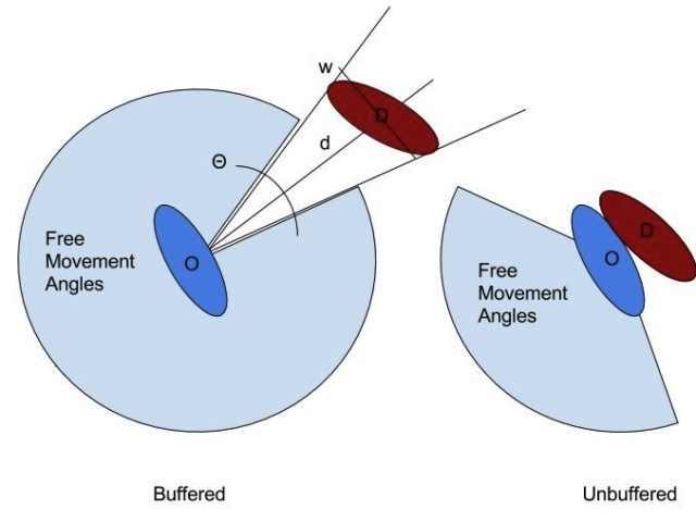
Figure 10 – A trigonometric demonstration of angle-constraint applied by a “bodying” defender.

The model we used for buffering assumed that both players could summon ideal, unhindered accelerations.  But the defense does not strictly need perfect acceleration as long as the offense does not enjoy it either.  If the defender proactively closes the buffer completely, the exponential model no longer applies; the offense will abut up against the defense halfway through his first stride.  This changes the nature of the game to one of footwork, strength and balance; the offense must out-manouevre the defense and regain separation first.

As above, the advantage (illustrated in Figure 10) can be loosely quantified using mathematical arguments. The useful angle (in radians) of free acceleration can be loosely described as:

Θ = 2π – 2arctan(w/2d)

Where d is the distance between the two bodies, and w is the planar width of the defender presented to the cutter (a maximum of the defender’s elbow-to-elbow breadth). As w/2d approaches zero, the available angles shrink to 180° (in practice, it shrinks to less than this, because humans are highly anisotropic, and they just can’t accelerate effectively in all directions without first turning their hips).

The risk that the defense willingly accepts in this case is the danger that the cutter might step back quickly enough and outflank him or, may summon the strength to just drive past the defender’s shoulder.  That is, if the cutter regains enough space to accelerate, the competition switches back to the mathematical models cited earlier. But now, the defense has already gambled away the buffers calculated earlier, and most likely won’t be able to recover.

The Balance

The two modes of defense herein described, buffering and bodying, should be viewed as complementary methods; good defenders must be able to use both competently, and be able to slide seamlessly between them as circumstances dictate.

The defense should buffer when

• the cutter has few, predictable cutting options
• the threatening spaces are large, and in mostly one area
• the cutter is unlikely to get a direct pass
• the cutter is agile or physically, but not a fast sprinter

The defense should body or jockey when

• the cutter has several cutting options
• the threatening spaces are small, but in several directions
• the cutter could be a target for a direct pass
• the cutter is a fast sprinter, but less agile and less strong

Although it is rare to be equally good at both modes of defense, all defenders must know how to use both modes, how their natural strengths might predispose them one way or the other, and their limitations. By applying math to your reasoning, you can better identify and articulate your personal optimum.

*NB: exp(a+b) = exp(a)exp(b)